│   collinear_dataset.py
│   compare_time.py
│   contour_plot.gif
│   degreevstheta.py
│   gif1.gif
│   gif2.gif
│   linear_regression_test.py
│   line_plot.gif
│   Makefile
│   metrics.py
│   Normal_regression.py
│   plot_contour.py
│   poly_features_test.py
│   README.md
│   surface_plot.gif
│
├───images
│       q5plot.png
│       q6plot.png
│       q8features.png
│       q8samples.png
│
├───linearRegression
│   │   linearRegression.py
│   │   __init__.py
│   │
│   └───__pycache__
│           linearRegression.cpython-37.pyc
│           __init__.cpython-37.pyc
│
├───preprocessing
│   │   polynomial_features.py
│   │   __init__.py
│   │
│   └───__pycache__
│           polynomial_features.cpython-37.pyc
│           __init__.cpython-37.pyc
│
├───temp_images
└───__pycache__
        metrics.cpython-37.pyc
make help
make regression
make polynomial_features
make normal_regression
make poly_theta
make contour
make compare_time
make collinear
-
Learning rate type = constant RMSE: 0.9119624181584616 MAE: 0.7126923090787688
-
Learning rate type = inverse RMSE: 0.9049599308106121 MAE: 0.7098334683036919
-
Learning rate type = constant RMSE: 0.9069295672718122 MAE: 0.7108301179089876
-
Learning rate type = inverse RMSE: 0.9607329070540364 MAE: 0.7641616657610887
-
Learning rate type = constant RMSE: 0.9046502501334435 MAE: 0.7102161700019564
-
Learning rate type = inverse RMSE: 0.9268357442221973 MAE: 0.7309246821952116
-
The output [[1, 2]] is [[1, 1, 2, 1, 2, 4]]
-
The output for [[1, 2, 3]] is [[1, 1, 2, 3, 1, 2, 3, 4, 6, 9]]
-
The outputs are similar to sklearn's PolynomialFeatures fit transform
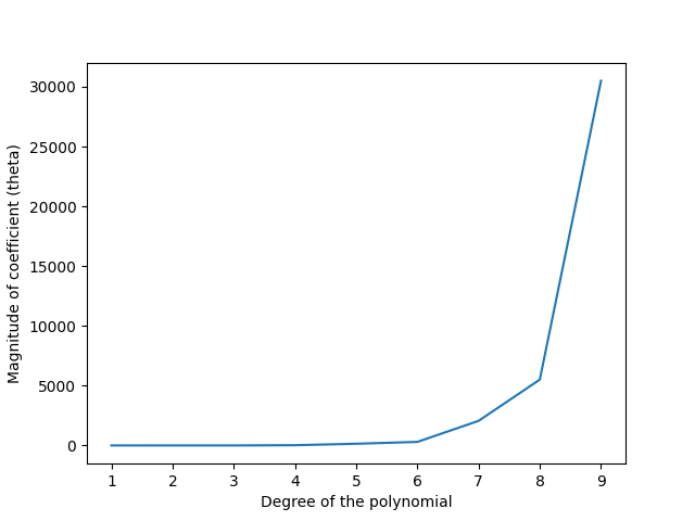
- Conclusion - As the degree of the polynomial increases, the norm of theta increases because of overfitting.
Conclusion
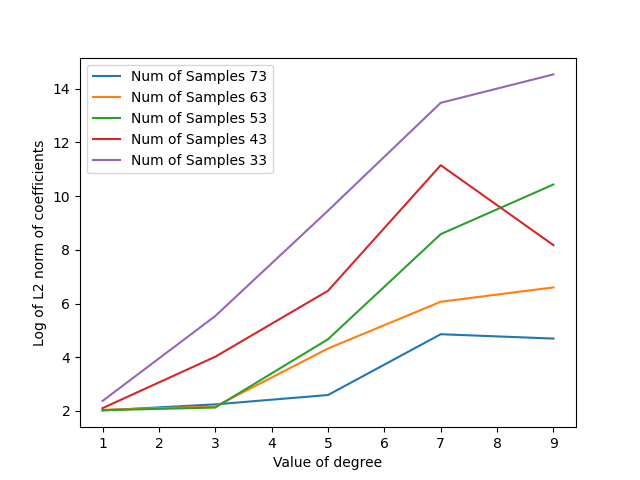
- As the degree increases magnitude of theta increases due to overfitting of data.
- But at the same degree, as the number of samples increases, the magnitude of theta decreases because more samples reduce the overfitting to some extent.


- Theoretical time complexity of Normal equation is O(D^2N) + O(D^3)
- Theoretical time complexity of Gradient Descent equation is O((t+N)D^2)
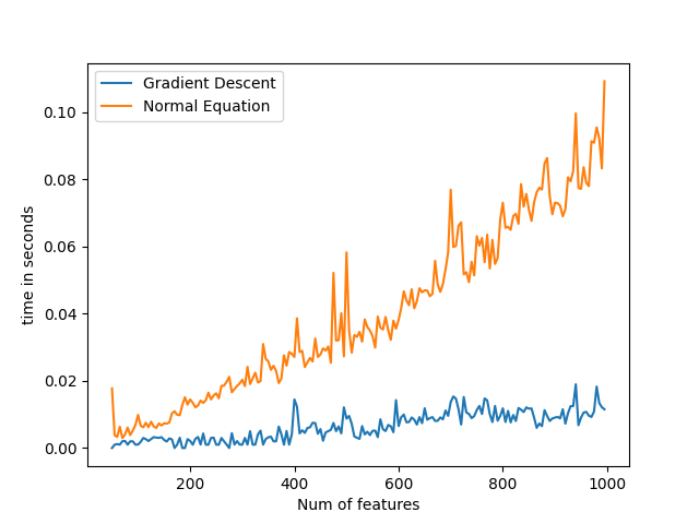
When the number of samples are kept constant, normal equation solution takes more time as it has a factor of D^3 whereas Gradient Descent has a factor of D^2 in the time complexity.
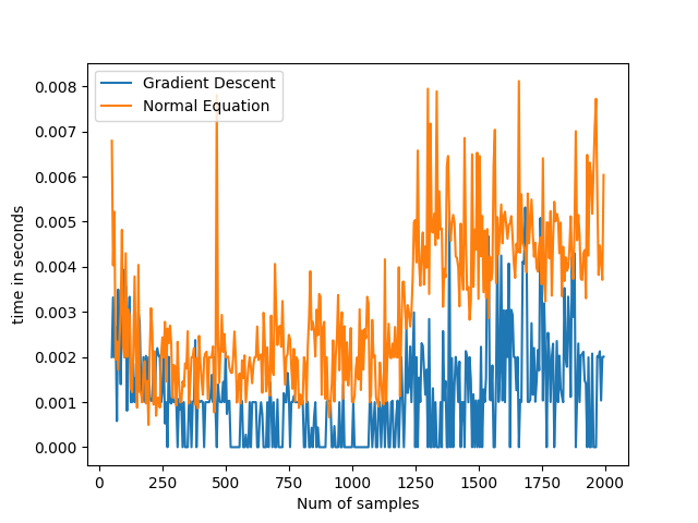
When the number of features are kept constant varying number of samples, it can be noticed that time for normal equation is still higher as compared to gradient descent because of computational expenses.
- The gradient descent implementation works for the multicollinearity.
- But as the multiplication factor increases, RMSE and MAE values takes a large shoot
- It reduces the precision of the coefficients