**MLP、CNN、ResNet **


X = []
lbl = []
for mod in mods:
    for snr in snrs:
        X.append(Xd[(mod,snr)])
        for i in range(Xd[(mod,snr)].shape[0]):
            lbl.append((mod,snr))
X = np.vstack(X)
file.close()
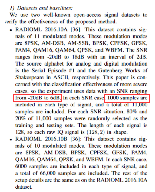
上述论文的分类任务是识别和区分不同类型的无线电调制方式。
项目地址:https://github.com/daetz-coder/RadioML2016.10a_CNN

数据链接:https://pan.baidu.com/s/1sxyWf4M0ouAloslcXSJe9w?pwd=2016
提取码:2016
下面介绍具体的处理方式,首先为了方便数据加载,根据SNR的不同划分为多个csv子文件
import pickle
import pandas as pd

# 指定pickle文件路径
pickle_file_path = './data/RML2016.10a_dict.pkl'

# 加载数据
with open(pickle_file_path, 'rb') as file:
    data_dict = pickle.load(file, encoding='latin1')

# 创建一个字典,用于按SNR组织数据
data_by_snr = {}

# 遍历数据字典,将数据按SNR分组
for key, value in data_dict.items():
    mod_type, snr = key
    if snr not in data_by_snr:
        data_by_snr[snr] = {}
    if mod_type not in data_by_snr[snr]:
        data_by_snr[snr][mod_type] = []
    # 只保留1000条数据
    data_by_snr[snr][mod_type].extend(value[:1000])

# 创建并保存每个SNR对应的CSV文件
for snr, mod_data in data_by_snr.items():
    combined_df = pd.DataFrame()
    for mod_type, samples in mod_data.items():
        for sample in samples:
            flat_sample = sample.flatten()
            temp_df = pd.DataFrame([flat_sample], columns=[f'Sample_{i}' for i in range(flat_sample.size)])
            temp_df['Mod_Type'] = mod_type
            temp_df['SNR'] = snr
            combined_df = pd.concat([combined_df, temp_df], ignore_index=True)

    # 保存到CSV文件
    csv_file_path = f'output_data_snr_{snr}.csv'
    combined_df.to_csv(csv_file_path, index=False)
    print(f"CSV file saved for SNR {snr}: {csv_file_path}")

print("Data processing complete. All CSV files saved.")import torch
import torch.nn as nn
import torch.optim as optim
from torch.utils.data import DataLoader, TensorDataset, random_split
import pandas as pd
import numpy as np
import matplotlib.pyplot as plt
from sklearn.metrics import confusion_matrix, ConfusionMatrixDisplay
# 加载数据
csv_file_path = 'snr_data/output_data_snr_6.csv'
data_frame = pd.read_csv(csv_file_path)
# 提取前256列数据并转换为张量
vectors = torch.tensor(data_frame.iloc[:, :256].values, dtype=torch.float32)
# 划分训练集和测试集索引
train_size = int(0.8 * len(vectors))
test_size = len(vectors) - train_size
train_indices, test_indices = random_split(range(len(vectors)), [train_size, test_size])
# 使用训练集的统计量进行归一化
train_vectors = vectors[train_indices]
train_mean = train_vectors.mean(dim=0, keepdim=True)
train_std = train_vectors.std(dim=0, keepdim=True)
vectors = (vectors - train_mean) / train_std
# 转置和重塑为16x16 若MLP 无需重构
vectors = vectors.view(-1, 16, 16).unsqueeze(1).permute(0, 1, 3, 2) # 添加通道维度并进行转置
# 提取Mod_Type列并转换为数值标签
mod_types = data_frame['Mod_Type'].astype('category').cat.codes.values
labels = torch.tensor(mod_types, dtype=torch.long)
# 创建TensorDataset
dataset = TensorDataset(vectors, labels)
# 创建训练集和测试集
train_dataset = TensorDataset(vectors[train_indices], labels[train_indices])
test_dataset = TensorDataset(vectors[test_indices], labels[test_indices])
# 创建DataLoader
train_loader = DataLoader(train_dataset, batch_size=32, shuffle=True)
test_loader = DataLoader(test_dataset, batch_size=32, shuffle=False)这里需要加载具体模型
criterion = nn.CrossEntropyLoss()
optimizer = optim.Adam(model.parameters(), lr=0.001)
num_epochs = 100
train_losses = []
test_losses = []
train_accuracies = []
test_accuracies = []
def calculate_accuracy(outputs, labels):
_, predicted = torch.max(outputs, 1)
total = labels.size(0)
correct = (predicted == labels).sum().item()
return correct / total
for epoch in range(num_epochs):
# 训练阶段
model.train()
running_loss = 0.0
correct = 0
total = 0
for inputs, labels in train_loader:
optimizer.zero_grad()
outputs = model(inputs)
loss = criterion(outputs, labels)
loss.backward()
optimizer.step()
running_loss += loss.item()
correct += (outputs.argmax(1) == labels).sum().item()
total += labels.size(0)
train_loss = running_loss / len(train_loader)
train_accuracy = correct / total
train_losses.append(train_loss)
train_accuracies.append(train_accuracy)
# 测试阶段
model.eval()
running_loss = 0.0
correct = 0
total = 0
with torch.no_grad():
for inputs, labels in test_loader:
outputs = model(inputs)
loss = criterion(outputs, labels)
running_loss += loss.item()
correct += (outputs.argmax(1) == labels).sum().item()
total += labels.size(0)
test_loss = running_loss / len(test_loader)
test_accuracy = correct / total
test_losses.append(test_loss)
test_accuracies.append(test_accuracy)
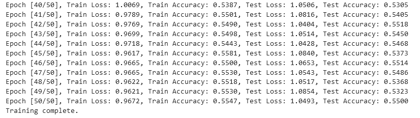
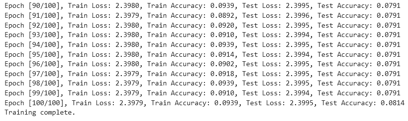
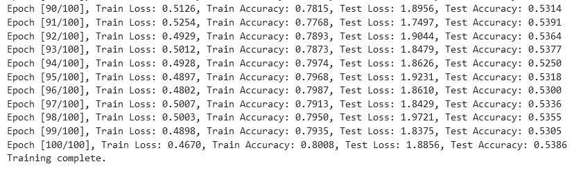
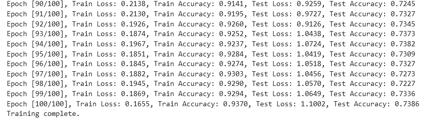
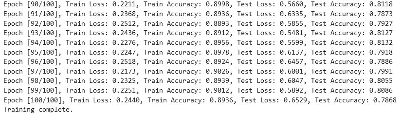
print(f"Epoch [{epoch+1}/{num_epochs}], Train Loss: {train_loss:.4f}, Train Accuracy: {train_accuracy:.4f}, Test Loss: {test_loss:.4f}, Test Accuracy: {test_accuracy:.4f}")
print("Training complete.")
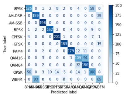
# 计算混淆矩阵
all_labels = []
all_predictions = []
model.eval()
with torch.no_grad():
for inputs, labels in test_loader:
outputs = model(inputs)
_, predicted = torch.max(outputs, 1)
all_labels.extend(labels.numpy())
all_predictions.extend(predicted.numpy())
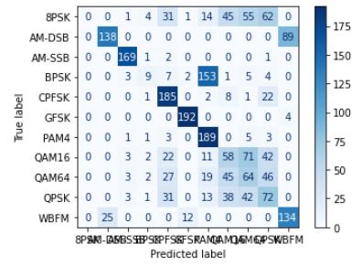
# 绘制混淆矩阵
cm = confusion_matrix(all_labels, all_predictions)
disp = ConfusionMatrixDisplay(confusion_matrix=cm, display_labels=data_frame['Mod_Type'].astype('category').cat.categories)
disp.plot(cmap=plt.cm.Blues)
plt.show()from torchinfo import summary
class SimpleNN(nn.Module):
def __init__(self):
super(SimpleNN, self).__init__()
self.fc1 = nn.Linear(256, 128)
self.fc2 = nn.Linear(128, 64)
self.fc3 = nn.Linear(64, 11) # 有11种调制类型
def forward(self, x):
x = torch.relu(self.fc1(x))
x = torch.relu(self.fc2(x))
x = self.fc3(x)
return x
model = SimpleNN()
# 打印模型结构和参数
summary(model, input_size=(1, 256))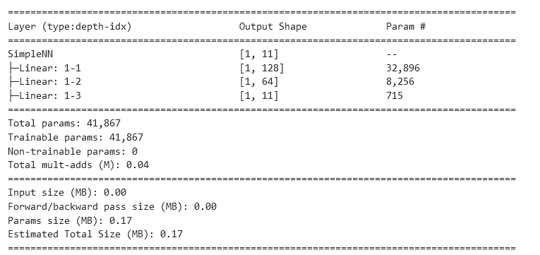


# 定义模型
from torchinfo import summary
class SimpleCNN(nn.Module):
    def __init__(self):
        super(SimpleCNN, self).__init__()
        self.conv1 = nn.Conv2d(1, 16, kernel_size=3, padding=1)
        self.bn1 = nn.BatchNorm2d(16)
        self.conv2 = nn.Conv2d(16, 32, kernel_size=3, padding=1)
        self.bn2 = nn.BatchNorm2d(32)
        self.dropout = nn.Dropout(0.3)
        self.fc1 = nn.Linear(32*4*4, 128)
        self.fc2 = nn.Linear(128, 64)
        self.fc3 = nn.Linear(64, 11)  # 11种调制类型

    def forward(self, x):
        x = torch.relu(self.bn1(self.conv1(x)))
        x = torch.max_pool2d(x, 2)
        x = torch.relu(self.bn2(self.conv2(x)))
        x = torch.max_pool2d(x, 2)
        x = x.view(x.size(0), -1)
        x = torch.relu(self.fc1(x))
        x = self.dropout(x)
        x = torch.relu(self.fc2(x))
        x = self.dropout(x)
        x = self.fc3(x)
        return x

model = SimpleCNN()
summary(model, input_size=(1, 1,16,16))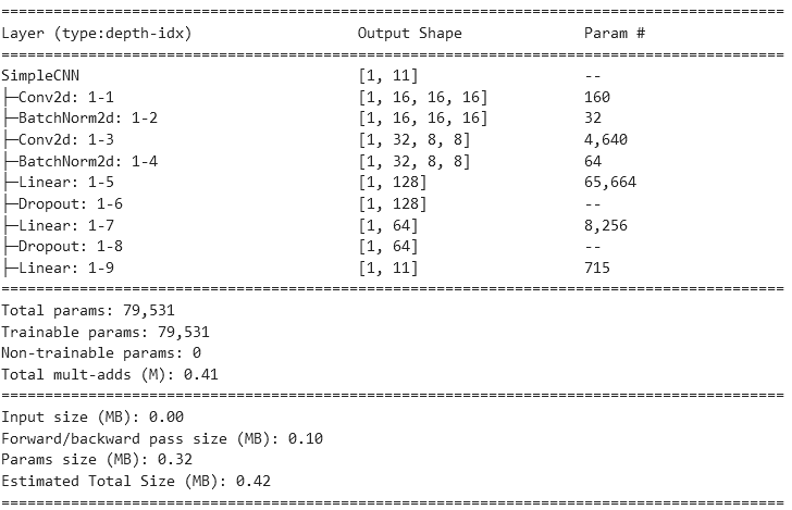

# 定义ResNet基本块
from torchinfo import summary
class BasicBlock(nn.Module):
    expansion = 1

    def __init__(self, in_planes, planes, stride=1):
        super(BasicBlock, self).__init__()
        self.conv1 = nn.Conv2d(in_planes, planes, kernel_size=3, stride=stride, padding=1, bias=False)
        self.bn1 = nn.BatchNorm2d(planes)
        self.conv2 = nn.Conv2d(planes, planes, kernel_size=3, stride=1, padding=1, bias=False)
        self.bn2 = nn.BatchNorm2d(planes)
        self.shortcut = nn.Sequential()
        if stride != 1 or in_planes != self.expansion * planes:
            self.shortcut = nn.Sequential(
                nn.Conv2d(in_planes, self.expansion * planes, kernel_size=1, stride=stride, bias=False),
                nn.BatchNorm2d(self.expansion * planes)
            )

    def forward(self, x):
        out = torch.relu(self.bn1(self.conv1(x)))
        out = self.bn2(self.conv2(out))
        out += self.shortcut(x)
        out = torch.relu(out)
        return out

# 定义ResNet
class ResNet(nn.Module):
    def __init__(self, block, num_blocks, num_classes=11):
        super(ResNet, self).__init__()
        self.in_planes = 16

        self.conv1 = nn.Conv2d(1, 16, kernel_size=3, stride=1, padding=1, bias=False)
        self.bn1 = nn.BatchNorm2d(16)
        self.layer1 = self._make_layer(block, 16, num_blocks[0], stride=1)
        self.layer2 = self._make_layer(block, 32, num_blocks[1], stride=2)
        self.linear = nn.Linear(32*4*4*4, num_classes)

    def _make_layer(self, block, planes, num_blocks, stride):
        strides = [stride] + [1]*(num_blocks-1)
        layers = []
        for stride in strides:
            layers.append(block(self.in_planes, planes, stride))
            self.in_planes = planes * block.expansion
        return nn.Sequential(*layers)

    def forward(self, x):
        out = torch.relu(self.bn1(self.conv1(x)))
        out = self.layer1(out)
        out = self.layer2(out)
        out = torch.flatten(out, 1)
        out = self.linear(out)
        return out

def ResNet18():
    return ResNet(BasicBlock, [2, 2])

model = ResNet18()
summary(model, input_size=(1, 1,16,16))

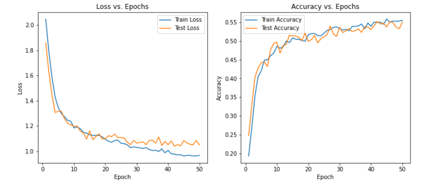
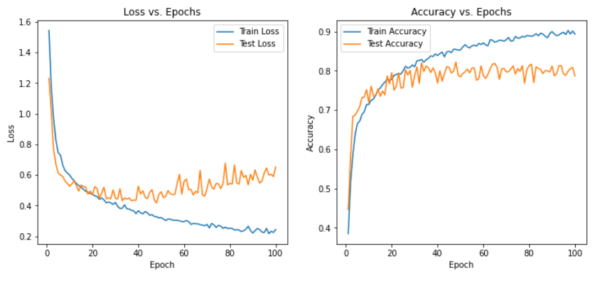
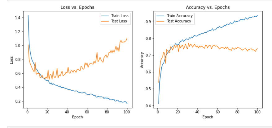
可以发现在三种模型下非常容易过拟合,为了探究是否是SNR的造成的影响,故修改SNR数值,进行下述实验
根据SNR的计算公式来看,-20db表示噪声的功率是信号的100倍,其余以此类推


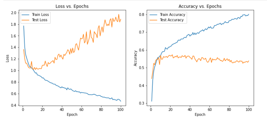
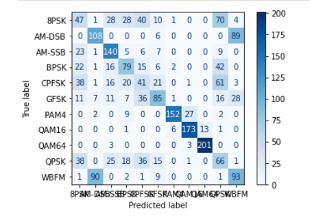
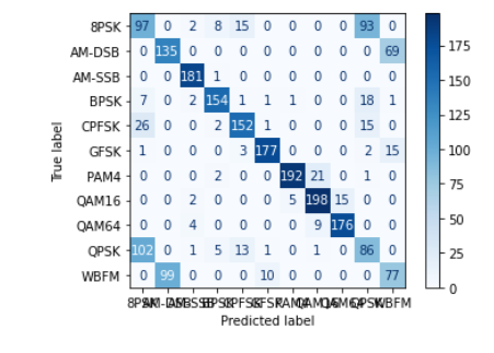


从实验结果来看,趋势还是比较符合预期,总体上SNR越大检测的性能越好,尤其是当SNR=-20db时无法区分任何一种类型
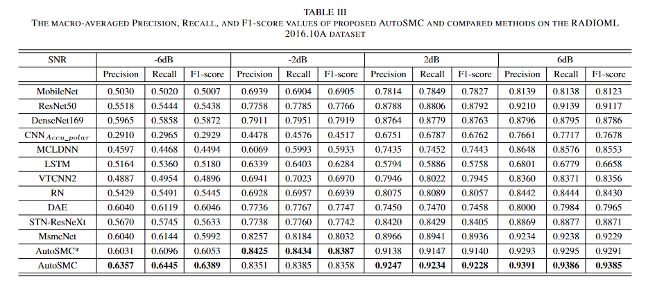
AutoSMC: An Automated Machine Learning Framework for Signal Modulation Classification

根据实验结果来看,在-6dB的表现情况在60%左右,6bB下在93%左右
在之前的两篇文章中仅仅是对数据直接重构分析,忽略了IQ分量应该共同进行描述描述
本篇内容在于介绍并利用IQ分量,并介绍IQ分量的其他表达方式
在无线通信中,信号通常表达为复数形式,这就是所谓的 I/Q 格式,其中:
- I 代表 In-phase 分量,即信号的实部。
- Q 代表 Quadrature 分量,即信号的虚部,与 I 分量正交(相位差 90 度)。
这种表示法使得信号可以在同一频带内携带更多的信息,并且有效地描述信号的振幅和相位,这对于调制和解调技术至关重要。
- 容量增加:使用 I 和 Q 两个正交分量,可以在同一频带宽度内传输双倍的数据,提高频谱效率。
- 信号处理的灵活性:I/Q 表示法可以方便地实施各种信号处理技术,如调制、解调、滤波和频谱分析。
- 支持多种调制方案:利用 I 和 Q 分量,可以实现各种调制技术,包括最常用的 QAM、QPSK 等。
- 精确表达信号:I/Q 数据能够精确描述信号的变化,包括幅度和相位的变化,这对于通信系统中信号的恢复非常重要。
从 I/Q 数据还原原始波形,主要是将这些复数数据转换为时域信号。这可以通过以下数学公式进行:
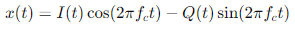
这个公式显示了如何将 I 分量与余弦波(同相位)和 Q 分量与正弦波(正交相位)相乘后相减,从而构造出时域中的原始信号。
傅里叶变换是将时域信号转换为频域信号的过程。对于 I/Q 数据,可以分别对 I 和 Q 分量进行傅里叶变换:
- 对 I 和 Q 分量进行离散傅里叶变换(DFT):这通常通过快速傅里叶变换(FFT)算法实现。
- 解析频谱:对 I 和 Q 分量的变换结果可以组合起来分析整个信号的频谱特性。
例如,使用 NumPy 进行 FFT 可以这样实现:
import numpy as np
I = np.array(...)  # I 分量
Q = np.array(...)  # Q 分量
complex_signal = I + 1j*Q  # 构建复数信号
fft_result = np.fft.fft(complex_signal) # 对复数信号进行 FFTimport pandas as pd
import numpy as np
# 加载数据
df = pd.read_csv("output_data_multi.csv")
# 提取 I 和 Q 分量
I_components = df.loc[:, "Sample_0":"Sample_127"].values # 前128个样本为I分量
Q_components = df.loc[:, "Sample_128":"Sample_255"].values # 接下来128个样本为Q分量
# 重构数据为复数形式,其中 I 为实部,Q 为虚部
complex_data = I_components + 1j * Q_components
# 保留调制类型和信噪比信息
mod_type = df["Mod_Type"]
snr = df["SNR"]
# 现在 complex_data 是一个包含复数信号的 NumPy 数组,mod_type 和 snr 是 Series 对象包含对应的调制类型和信噪比信息
complex_data[:1]array([[-5.90147120e-03-0.00779554j, -2.34581790e-03-0.00781637j,
-7.45061260e-04-0.00401967j, -5.34572450e-03-0.00511351j,
-5.78941800e-03-0.00593952j, -3.69683500e-03-0.0065699j ,
-4.97868750e-03-0.00558479j, -6.56572800e-03-0.00529769j,
-9.04932200e-03+0.00021024j, -4.83668640e-03-0.00604725j,
-1.00837140e-02-0.00705299j, -4.53815700e-03-0.00768376j,
-4.31498840e-03-0.00682943j, -5.13423300e-03-0.00526323j,
-6.07567300e-03-0.00428441j, 1.18665890e-03-0.00823529j,
-4.65670100e-03-0.00887949j, -6.95332750e-03-0.00665625j,
-6.66823420e-03-0.00873265j, -6.43977240e-03-0.00415313j,
-3.82532270e-03-0.00815829j, -8.38821850e-03-0.00602711j,
-1.01344110e-02-0.01298266j, -6.90073200e-03-0.00686788j,
-9.62839300e-03-0.00674923j, -1.55354580e-03-0.00403722j,
-2.88469440e-03-0.00778409j, -4.51788800e-03-0.00531385j,
3.41027650e-03+0.00321187j, 7.41052260e-03-0.00500479j,
3.35769330e-03+0.00121511j, 7.62627900e-03+0.00072439j,
8.82679400e-03+0.00443489j, 3.42824610e-03+0.0083125j ,
1.84084000e-03+0.00883208j, 6.41621460e-03+0.0059255j ,
-1.63305740e-04+0.00833821j, -2.24135860e-03+0.00718797j,
-5.19226260e-03+0.00816119j, -3.63920980e-03+0.00870452j,
-1.01316330e-02+0.00650418j, -6.39987200e-03+0.00439436j,
-6.06458450e-03+0.00282486j, -7.66557640e-03+0.00216367j,
-3.44835570e-03+0.00520329j, 4.42530580e-04+0.00740604j,
2.56719800e-03+0.00053031j, 4.74520000e-03+0.00502639j,
4.66336500e-03+0.00479635j, 6.47741840e-03+0.00892057j,
8.53952900e-03+0.00727959j, 4.98457070e-03+0.00410889j,
1.83550680e-04-0.00164091j, 2.53180620e-04+0.00032166j,
-2.90070500e-03-0.00435043j, -5.35907460e-03-0.00534027j,
-9.30814800e-03-0.00672173j, -5.05294140e-03-0.00410643j,
-4.83987950e-03-0.00531335j, 1.17973956e-04-0.00456619j,
-5.48875540e-04-0.00476122j, 8.79733360e-04-0.00262099j,
6.80832940e-03+0.00264574j, 8.02225800e-03+0.00791668j,
8.17798450e-03+0.00810155j, 6.84361200e-03+0.00856092j,
3.34831540e-03+0.00586885j, 2.62019620e-03+0.0090829j ,
-2.50967550e-03+0.00278104j, -6.09290500e-04-0.00458179j,
-8.00378100e-03-0.00078458j, -1.06874220e-02+0.00190195j,
-8.18693600e-03-0.00514773j, -9.52030600e-03-0.00967547j,
-4.64970530e-03-0.00738798j, -1.15614310e-03-0.00874938j,
2.20692440e-03-0.00441817j, 4.98547300e-03-0.00172313j,
2.16765120e-03-0.00309234j, 6.35635430e-03-0.0008443j ,
1.04583080e-02+0.00702607j, 7.48503440e-03+0.00947603j,
6.23615830e-03+0.00366654j, 2.93730760e-03+0.00918464j,
1.16433020e-03+0.00436038j, 2.31683560e-04+0.00822378j,
-4.89262350e-03+0.00838072j, -3.32372940e-03+0.0072375j ,
-6.60865700e-03+0.00306395j, -4.91313600e-03+0.00747482j,
-7.29229100e-03+0.00292273j, -6.01531470e-03+0.00505259j,
-1.28758220e-03+0.00033149j, 4.22199520e-04+0.00930912j,
2.63322060e-04+0.00462913j, 3.07579040e-03+0.00658605j,
3.98740960e-03+0.00548608j, 3.42952720e-03+0.00639373j,
2.69522470e-03+0.00506808j, 7.13837430e-03+0.00556591j,
6.24447500e-03+0.00681962j, 6.12162850e-03+0.0091046j ,
5.42381820e-03+0.00839265j, 1.00702720e-03+0.00871987j,
9.82678100e-04+0.01014247j, 1.36985770e-03+0.00758515j,
3.53600270e-03+0.00481515j, 4.30495700e-03+0.00565554j,
8.39837300e-03+0.00265674j, 8.00060500e-03-0.00235612j,
6.66820200e-03-0.00501084j, 8.24876000e-03-0.00279375j,
6.43996850e-03-0.00482372j, 1.07639670e-02-0.00445632j,
6.80366070e-03-0.00213765j, 2.71986000e-03-0.00170917j,
6.70633800e-05-0.00275444j, 2.20027730e-03-0.00213406j,
9.56511500e-04-0.00033254j, -1.03281380e-03-0.00055647j,
-5.32025420e-03+0.00808902j, -7.41181000e-03+0.00666311j,
-7.29165800e-03+0.00731658j, 1.09607930e-04+0.00554266j,
-3.40843060e-03+0.00534808j, -3.26823540e-03+0.01032196j,
-3.04144340e-03+0.00841506j, 5.69031200e-03+0.00544548j]])import numpy as np
import matplotlib.pyplot as plt
# 参数设置
fs = 200e3 # 采样率,200kHz
fc = 100e3 # 假设的载波频率,可以根据实际情况调整
t = np.arange(128) / fs # 生成时间数组,对于每个样本128个点
# 生成载波
cos_wave = np.cos(2 * np.pi * fc * t) # 余弦载波
sin_wave = np.sin(2 * np.pi * fc * t) # 正弦载波
df = pd.read_csv("output_data_multi.csv")
# 提取 I 和 Q 分量
I_components = df.loc[:, "Sample_0":"Sample_127"].values # 前128个样本为I分量
Q_components = df.loc[:, "Sample_128":"Sample_255"].values # 接下来128个样本为Q分量
# 重构数据为复数形式,其中 I 为实部,Q 为虚部
complex_data = I_components + 1j * Q_components
# 选择一个样本进行还原,这里假设选择第一个样本
sample_signal = complex_data[0]
# 还原信号
restored_signal = np.real(sample_signal) * cos_wave - np.imag(sample_signal) * sin_wave
# 绘制还原的信号
plt.figure(figsize=(10, 5))
plt.plot(t, restored_signal, label='Restored Signal')
plt.title('Restored Signal from I/Q Components')
plt.xlabel('Time (seconds)')
plt.ylabel('Amplitude')
plt.legend()
plt.show()
import pandas as pd
import numpy as np
import matplotlib.pyplot as plt
# 加载数据
df = pd.read_csv("output_data_multi.csv")

# 提取 I 和 Q 分量
I_components = df.loc[:, "Sample_0":"Sample_127"].values  # 前128个样本为I分量
Q_components = df.loc[:, "Sample_128":"Sample_255"].values  # 接下来128个样本为Q分量

# 重构数据为复数形式,其中 I 为实部,Q 为虚部
complex_data = I_components + 1j * Q_components

# 保留调制类型和信噪比信息
mod_type = df["Mod_Type"]
snr = df["SNR"]

# 我们取第一个样本来进行FFT
sample_signal = complex_data[1]

# 对该样本进行快速傅里叶变换
fft_result = np.fft.fft(sample_signal)

# 计算频率轴的刻度
n = len(sample_signal)
frequency = np.fft.fftfreq(n, d=1/200000)  # d 是采样间隔,对应的采样率是200kHz

# 绘制FFT结果的幅度谱
plt.figure(figsize=(12, 6))
plt.plot(frequency, np.abs(fft_result))
plt.title('Frequency domain of the signal')
plt.xlabel('Frequency (Hz)')
plt.ylabel('Amplitude')
plt.grid(True)
plt.show()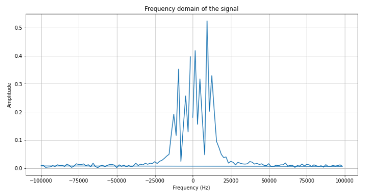
import numpy as np
import matplotlib.pyplot as plt

# 假设 complex_data 包含了多个信号样本,我们取第一个样本
sample_signal = complex_data[0]

# 生成时间轴
fs = 200000  # 采样率200kHz
t = np.arange(len(sample_signal)) / fs  # 时间向量

# 绘制时间域图
plt.figure(figsize=(12, 6))
plt.plot(t, np.real(sample_signal), label='Real Part')
plt.plot(t, np.imag(sample_signal), label='Imaginary Part', linestyle='--')
plt.title('Time Domain Signal')
plt.xlabel('Time (seconds)')
plt.ylabel('Amplitude')
plt.legend()
plt.grid(True)
plt.show()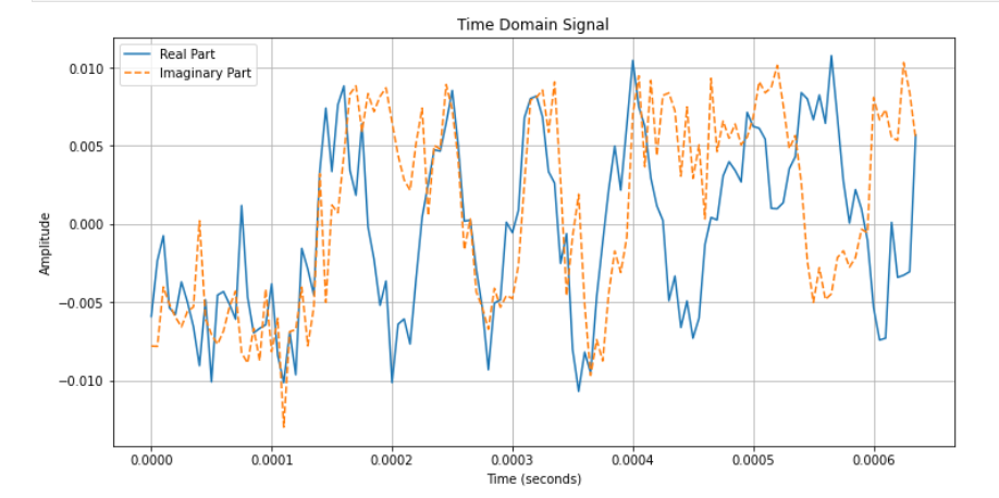
通过计算信号的傅里叶变换的平方的模来得到
# 对信号进行快速傅里叶变换
fft_result = np.fft.fft(sample_signal)

# 计算功率谱
power_spectrum = np.abs(fft_result)**2

# 生成频率轴
n = len(sample_signal)
frequency = np.fft.fftfreq(n, d=1/fs)

# 绘制功率谱图
plt.figure(figsize=(12, 6))
plt.plot(frequency, power_spectrum)
plt.title('Power Spectrum')
plt.xlabel('Frequency (Hz)')
plt.ylabel('Power')
plt.grid(True)
plt.xlim([0, fs/2])  # 通常只显示正频率部分直到Nyquist频率
plt.show()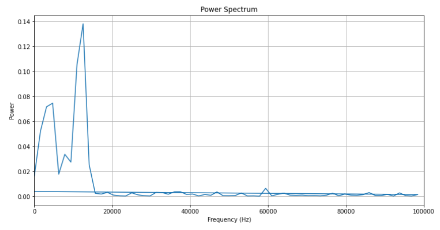
时间域图中,实部和虚部分别表示了信号的两个正交分量随时间的变化。
功率谱图中,每个频率点的幅度平方表示了该频率成分的能量或功率。通常我们只关注到Nyquist频率(采样率的一半)的正频率部分。
-
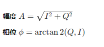
将 IQ (In-phase and Quadrature) 数据表示为单个值的一种常见方法是转换这些分量为幅度 (magnitude) 和相位 (phase)。这种表示有助于捕获信号的本质特性,尤其是在处理通信信号和频域分析时。幅度和相位能够提供关于信号强度和时间变化的信息,这在某些应用场景下比原始的 I 和 Q 分量更有用。
幅度 AAA 和相位 ϕ\phiϕ 可以从 I 和 Q 分量通过以下公式计算得出:
import torch

# 假设 I_components 和 Q_components 是包含 I 和 Q 数据的张量
I_components = torch.tensor(data_frame.iloc[:, :128].values, dtype=torch.float32)
Q_components = torch.tensor(data_frame.iloc[:, 128:256].values, dtype=torch.float32)

# 计算幅度和相位
magnitude = torch.sqrt(I_components**2 + Q_components**2)
phase = torch.atan2(Q_components, I_components)

# 可以选择只使用幅度或相位,或者将它们作为两个特征组合使用
features = torch.stack([magnitude, phase], dim=-1) # 按最后一个维度堆叠- 单一特征选择:如果您想使用单个值来表示 IQ 数据,可以选择使用幅度或相位中的一个。通常,幅度在许多应用中都是非常有用的信息,因为它直接反映了信号的强度。
- 特征工程:您可以根据应用的具体需要决定是否需要额外处理这些特征,例如通过标准化或归一化来调整它们的尺度。
- 模型输入:计算得到的幅度或相位可以直接用作机器学习模型的输入,尤其是在信号处理和通信系统分析中。
- 通信系统:在处理调制信号时,幅度和相位常常提供了比原始 I/Q 分量更直观的信号特征。
- 特征简化:在某些情况下,使用幅度或相位可以简化问题的复杂性,减少需要处理的数据量。
- 性能改进:在某些机器学习任务中,这种转换可能会改善模型的性能,因为它能够捕获信号的关键特性。
总之,通过转换 I 和 Q 分量为幅度和相位,您可以从另一个角度捕捉信号的特性,这可能对于特定的应用场景(如信号分类、检测或其他分析任务)非常有用。这种方法在许多通信领域和信号处理应用中都得到了广泛的使用。
# 提取 I 和 Q 分量
I_components = data_frame.iloc[:, :128].values
Q_components = data_frame.iloc[:, 128:256].values

# 将 I 和 Q 分量堆叠
stacked_components = np.stack((I_components, Q_components), axis=1)

# 转换为torch张量
vectors = torch.tensor(stacked_components, dtype=torch.float32) # 形状为 [n_samples, 2, 128]# 提取前256列数据并转换为张量
vectors = torch.tensor(data_frame.iloc[:, :256].values, dtype=torch.float32)# 提取 I 和 Q 分量
I_components = data_frame.iloc[:, :128].values
Q_components = data_frame.iloc[:, 128:256].values
# 计算幅度
magnitude = np.sqrt(I_components**2 + Q_components**2)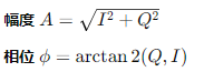
phase = np.arctan2(Q_components, I_components)
phase_tensor = torch.tensor(phase, dtype=torch.float32).unsqueeze(-1) # 添加特征维度magnitude = np.sqrt(I_components**2 + Q_components**2)
phase = np.arctan2(Q_components, I_components)
combined = np.stack((magnitude, phase), axis=-1) # 在特征维度上堆叠
combined_tensor = torch.tensor(combined, dtype=torch.float32)magnitude = np.sqrt(I_components**2 + Q_components**2)
phase = np.arctan2(Q_components, I_components)
flattened = np.concatenate((magnitude, phase), axis=1) # 在序列长度维度上连接
flattened_tensor = torch.tensor(flattened, dtype=torch.float32)给出其中的一种模型示例(SNR=6)
# 提取 I 和 Q 分量
I_components = data_frame.iloc[:, :128].values
Q_components = data_frame.iloc[:, 128:256].values

# 将 I 和 Q 分量堆叠
stacked_components = np.stack((I_components, Q_components), axis=1)

# 转换为torch张量
vectors = torch.tensor(stacked_components, dtype=torch.float32)  # 形状为 [n_samples, 2, 128]
class SimpleTransformer(nn.Module):
def __init__(self, input_dim, num_heads, num_layers, num_classes):
super(SimpleTransformer, self).__init__()
self.embedding = nn.Linear(128, input_dim) # 确保这里从128维映射到input_dim
encoder_layers = TransformerEncoderLayer(d_model=input_dim, nhead=num_heads)
self.transformer_encoder = TransformerEncoder(encoder_layer=encoder_layers, num_layers=num_layers)
self.fc_out = nn.Linear(input_dim, num_classes)
self.dropout = nn.Dropout(0.3)
def forward(self, x):
x = x.permute(1, 0, 2) # Rearrange input to seq_length, batch_size, features
x = self.embedding(x)
x = self.transformer_encoder(x)
x = x.mean(dim=0) # Aggregate over the sequence
x = self.dropout(x)
x = self.fc_out(x)
return x
# Model instantiation
model = SimpleTransformer(input_dim=16, num_heads=4, num_layers=2, num_classes=11)