torch-fem

Simple GPU accelerated differentiable finite elements for small-deformation solid mechanics with PyTorch. PyTorch enables efficient computation of sensitivities via automatic differentiation and using them in optimization tasks.

Installation

Your may install torch-fem via pip with

pip install torch-fem

Optional: For GPU support, install CUDA and the corresponding CuPy version with

pip install cupy-cuda11x # v11.2 - 11.8
pip install cupy-cuda12x # v12.x

Features

• Elements
  • 1D: Bar1, Bar2
  • 2D: Quad1, Quad2, Tria1, Tria2
  • 3D: Hexa1, Hexa2, Tetra1, Tetra2
  • Shell: Flat-facet triangle (linear only)
• Material models (3D, 2D plane stress, 2D plane strain, 1D)
  • Isotropic linear elasticity
  • Orthotropic linear elasticity
  • Isotropic plasticity
• Utilities
  • Homogenization of orthotropic stiffness
  • I/O to and from other mesh formats via meshio

Basic examples

The subdirectory examples->basic contains a couple of Jupyter Notebooks demonstrating the use of torch-fem for trusses, planar problems, shells and solids. You may click on the examples to check out the notebooks online.

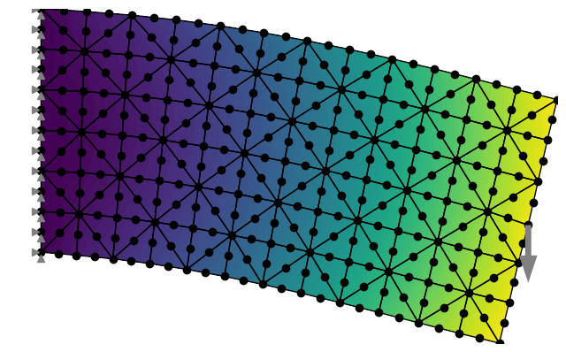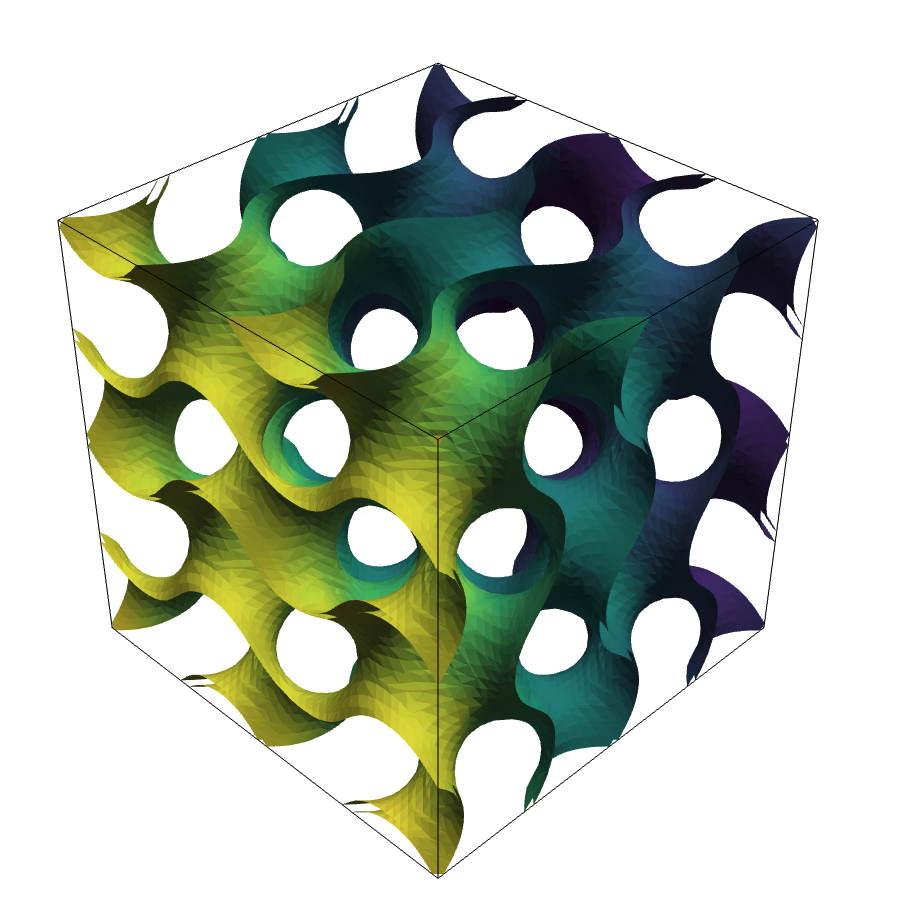
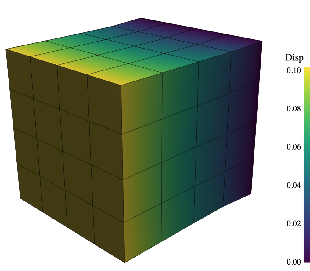
Gyroid: Support for voxel meshes and implicit surfaces.	Solid cubes: There are several examples with different element types rendered in PyVista.	Planar cantilever beams: There are several examples with different element types rendered in matplotlib.
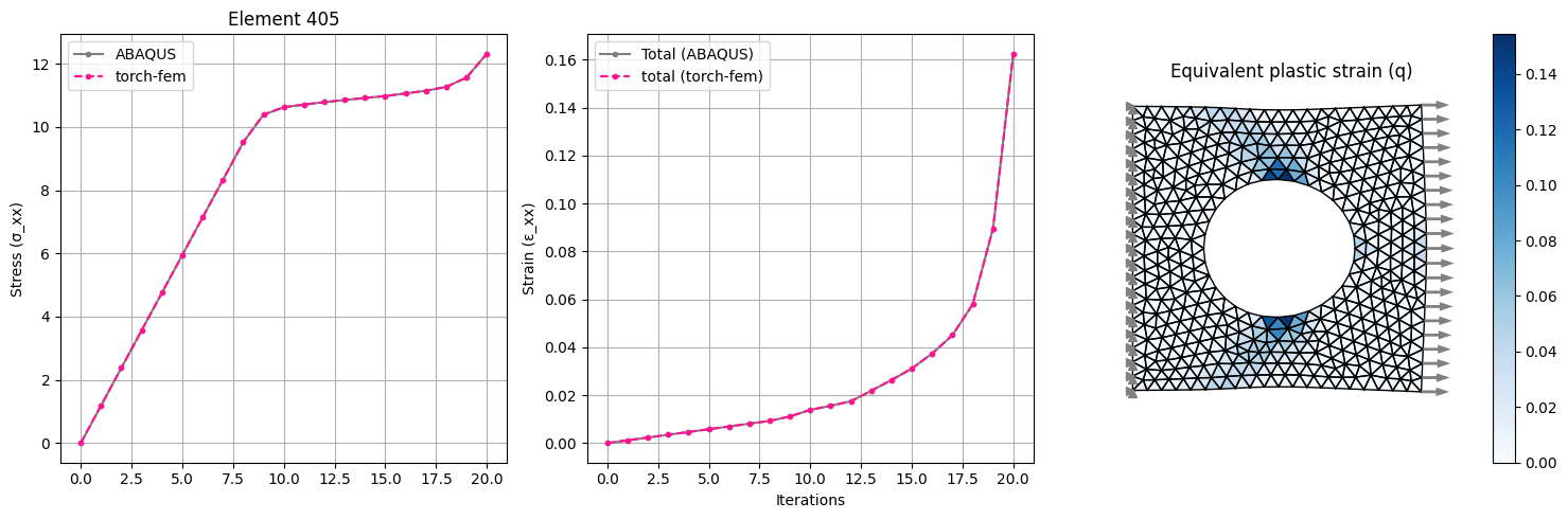
Plasticity in a plate with hole: Isotropic linear hardening model for plane-stress or plane-strain.

Optimization examples

The subdirectory examples->optimization demonstrates the use of torch-fem for optimization of structures (e.g. topology optimization, composite orientation optimization). You may click on the examples to check out the notebooks online.

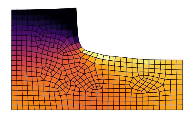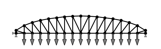
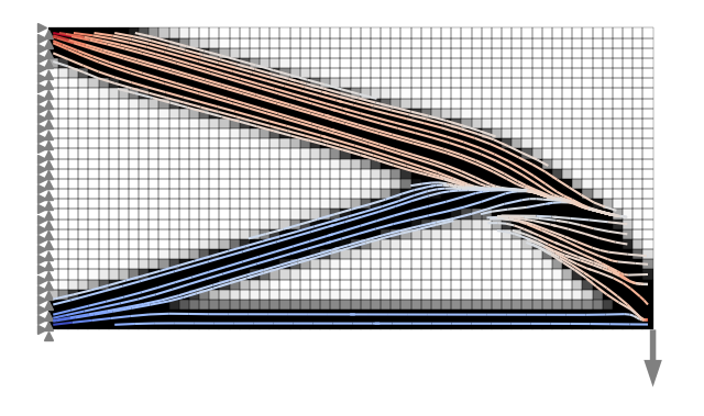
Shape optimization of a truss: The top nodes are moved and MMA + autograd is used to minimize the compliance.	Shape optimization of a fillet: The shape is morphed with shape basis vectors and MMA + autograd is used to minimize the maximum stress.
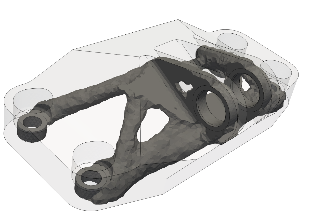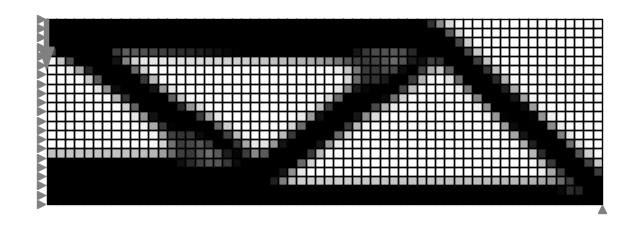
Topology optimization of a MBB beam: You can switch between analytical and autograd sensitivities.	Topology optimization of a jet engine bracket: The 3D model is exported to Paraview for visualization.
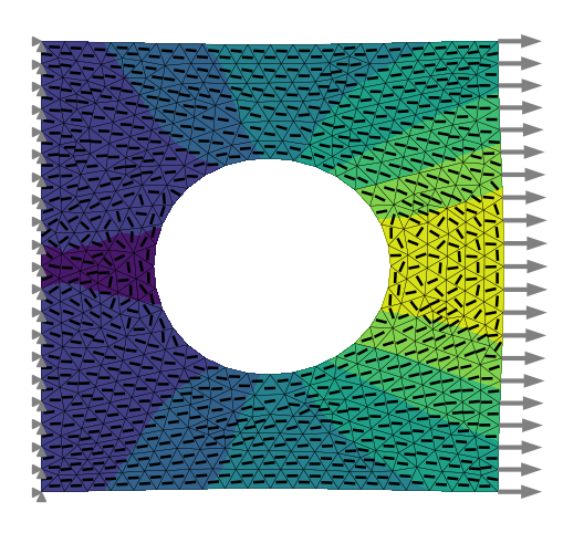
Combined topology and orientation optimization: Compliance is minimized by optimizing fiber orientation and density of an anisotropic material using automatic differentiation.	Fiber orientation optimization of a plate with a hole Compliance is minimized by optimizing the fiber orientation of an anisotropic material using automatic differentiation w.r.t. element-wise fiber angles.

Minimal example

This is a minimal example of how to use torch-fem to solve a very simple planar cantilever problem.

import torch
from torchfem import Planar
from torchfem.materials import IsotropicElasticityPlaneStress

torch.set_default_dtype(torch.float64)

# Material
material = IsotropicElasticityPlaneStress(E=1000.0, nu=0.3)

# Nodes and elements
nodes = torch.tensor([[0., 0.], [1., 0.], [2., 0.], [0., 1.], [1., 1.], [2., 1.]])
elements = torch.tensor([[0, 1, 4, 3], [1, 2, 5, 4]])

# Create model
cantilever = Planar(nodes, elements, material)

# Load at tip [Node_ID, DOF]
cantilever.forces[5, 1] = -1.0

# Constrained displacement at left end [Node_IDs, DOFs]
cantilever.constraints[[0, 3], :] = True

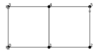
# Show model
cantilever.plot(node_markers="o", node_labels=True)

This creates a minimal planar FEM model:

# Solve
u, f, σ, ε, α = cantilever.solve()

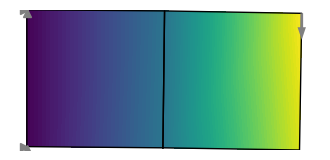
# Plot displacement magnitude on deformed state
cantilever.plot(u, node_property=torch.norm(u, dim=1))

This solves the model and plots the result:

If we want to compute gradients through the FEM model, we simply need to define the variables that require gradients. Automatic differentiation is performed through the entire FE solver.

# Enable automatic differentiation
cantilever.thickness.requires_grad = True
u, f, _, _, _ = cantilever.solve()

# Compute sensitivity of compliance w.r.t. element thicknesses
compliance = torch.inner(f.ravel(), u.ravel())
torch.autograd.grad(compliance, cantilever.thickness)[0]

Benchmarks

The following benchmarks were performed on a cube subjected to a one-dimensional extension. The cube is discretized with N x N x N linear hexahedral elements, has a side length of 1.0 and is made of a material with Young's modulus of 1000.0 and Poisson's ratio of 0.3. The cube is fixed at one end and a displacement of 0.1 is applied at the other end. The benchmark measures the forward time to assemble the stiffness matrix and the time to solve the linear system. In addition, it measures the backward time to compute the sensitivities of the sum of displacements with respect to forces.

Apple M1 Pro (10 cores, 16 GB RAM)

Python 3.10, SciPy 1.14.1, Apple Accelerate

N	DOFs	FWD Time	BWD Time	Peak RAM
10	3000	0.14s	0.03s	592.2MB
20	24000	0.99s	0.15s	968.3MB
30	81000	3.42s	0.57s	1562.8MB
40	192000	8.48s	1.14s	2497.1MB
50	375000	16.46s	2.23s	3963.7MB
60	648000	28.63s	3.56s	5503.3MB
70	1029000	46.86s	5.91s	6309.5MB
80	1536000	74.12s	10.69s	6933.7MB
90	2187000	121.11s	16.63s	7663.5MB
100	3000000	179.44s	38.35s	9662.4MB

AMD Ryzen Threadripper PRO 5995WX (64 Cores, 512 GB RAM) and NVIDIA GeForce RTX 4090

Python 3.12, CuPy 13.3.0, CUDA 11.8

N	DOFs	FWD Time	BWD Time	Peak RAM
10	3000	0.66s	0.15s	1371.7MB
20	24000	1.00s	0.43s	1358.9MB
30	81000	1.14s	0.65s	1371.1MB
40	192000	1.37s	0.83s	1367.3MB
50	375000	1.51s	1.04s	1356.4MB
60	648000	1.94s	1.43s	1342.1MB
70	1029000	5.19s	4.31s	1366.8MB
80	1536000	7.48s	18.88s	5105.6MB