-
Notifications
You must be signed in to change notification settings - Fork 350
SQL Performance Enhancement:IN Operator in WHERE Clause
【Abstract】
The essay analyzes the fundamental reason behind slow SQL statements and provides the solution to make improvements through code samples.
It is not uncommon to use the IN operator in WHERE statement. Such an example is the filtering operation by enumerated values, say, the customer age groups, by regions, or by orders.
An IN condition is usually written in the format of F IN (f1,…,fn). The condition is true when F field value is included in the set of values {fi,..}.
The computation of IN condition is slow because:
1. One to n comparisons between an F value and members of the set of values are needed when the left-to-right search is used to check whether F is contained in the set. Even if the binary search can be used when the set is ordered, a number of comparisons are still needed. The IN operator is thus extremely inefficient. The larger the set of values, the slower the computation;
2. The fields involved are often string type, which uses more storage space than integer type and which is slower in performing the comparison operation. A huge volume of data is commonly stored in the external storage devices. The IN computation is slow to both read in strings and compare them, particularly when a full-table traversal is involved.
First, we need to find the value range for IN field.
Usually there are only a few possible value ranges. Sometimes a code table, which we call dimension table, is created to store all possible values. Correspondingly, we call the to-be-queried table that contains the IN field the fact table.
If the IN field has a dimension table, its value range is already defined and no special handling is needed. If there isn’t a dimension table for it, we need to traverse the fact table to generate the value range, which is also called the field’s dimension table.
Whatever the dimension table already exists or it is generated later, it needs to be ordered by the set of values, so we can use the binary location (we will discuss it later) to speed up the subsequent computations.
Second, convert field values in the fact table into integers.
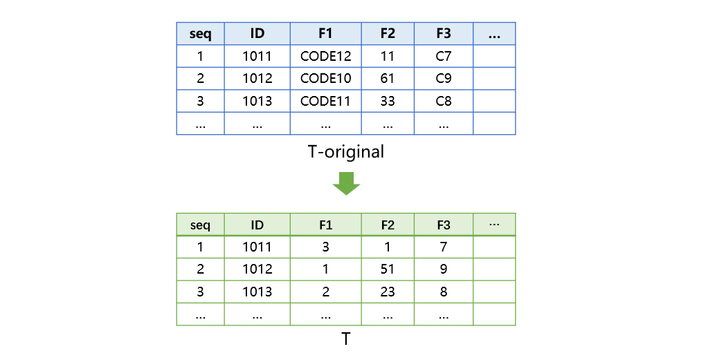
We traverse the IN field, find corresponding field values in the dimension table, replace IN field values with the sequence numbers of corresponding dimension items, and save the table as a new fact table. Generally a dimension table is not large and contains no greater than 65536 items (the sequence numbers are small integers).
Third, convert the set of IN field values {fi,..} into a Boolean dimension sequence.
In this step, we generate a Boolean sequence that is as long as the dimension table. Whether the ith member in the sequence is true is determined by whether the ith member of the dimension table is included in the set of values {fi,..}. If the latter is included in the set, the former is true; otherwise, the former is false. Such a sequence generated in this way is called Boolean dimension sequence.
Fourth, achieve the IN condition.
The query still requires a full traversal of the fact table, only without the need of comparison operation on the set of IN values. Since we have already converted the IN field values into sequence numbers of corresponding items in the dimension table, we can use the sequence numbers to get members of the Boolean dimension sequence. If a member retrieved is non-null, the field value is a target of the IN filtering condition; otherwise, the field value is not an eligible one.
Essentially, the method reduces computing time by converting “comparison of values of a set” into “the reference of sequence numbers”. Whatever the size of the set of IN field values, to achieve the filtering operation each field value will only need to reference a member of the Boolean dimension sequence according to the corresponding sequence number during the fact table traversal. The computing time is not connected to the number of enumerated IN values any more. It won’t increase as the number of enumerated IN values grows. The complexity degree of getting values by sequence numbers is far less than that of comparison of IN field values, and thus query performance is considerably improved.
Suppose the fact table is T, the SQL statement can be written as follows:
Select … from T where … F1 in (…) … F2 in (…) … F3 in (…) …
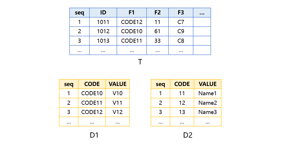
Below is the table’s data structure and its data. F1 field and F2 field have corresponding dimension tables. F3 field contains strings and does not have a corresponding dimension table.
Step 1: Get the value range of the IN field.
Create a dimension table for F3 using the following code:
| A | |
|---|---|
| 1 | =file("T-original.ctx").open().cursor('F3') |
| 2 | =A1.groups('F3') |
| 3 | =A2.new('F3':CODE) |
| 4 | =file("D3.btx").export@b(A3) |
A1: Open the source composite table T-original.ctx to get F3 field.
A2: Use groups function to group F3 field since the number of values in F3 is not large and return a result set ordered according to the order of F3.
Enclose F3 by single quotes to distinguish the field name from the namesake cell name. Single quotes are also used when a field name is the same as the variable name.
A3: Rename F3 CODE.
A4: Export A3’s result to D3.btx.
Note: F1 field and F2 field’s dimension tables D1 and D2 need to be ordered by CODE, too. If the original data is unordered, as sort function is needed to perform a pre-sort.
Step 2: Convert field values in the fact table into integers.
The following code converts values of fields F1, F2 and F3 in table T into sequence numbers in their corresponding dimension tables:
| A | B | |
|---|---|---|
| 1 | =file("T-original.ctx") | =file("T.ctx") |
| 2 | ["D1","D2","D3"] | =A2.(file(~/".btx").import@ib(CODE)) |
| 3 | =A1.open().cursor().run('F1'=B2(1).pos@b('F1'),'F2'=B2(2).pos@b('F2'),'F3'=B2(3).pos@b('F3')) | |
| 4 | =A1.reset@n(B1) | =B1.open().append@i(A3) |
A1,B1: Define the original composite table T-original.ctx and a new composite table file T.ctx respectively.
A2: Define the sequence of dimension tables to be converted.
B2: Open A2’s dimension table files in turn, retrieve data, and get the sequence of CODE field.
A3: Get all fields of A1’s table to define a cursor and convert values of F1, F2 and F3 fields into corresponding sequence numbers in the dimension tables.
A4: Create an empty composite table T.ctx having the same structure as the original composite table.
B4: Open the new T.ctx to append A3’s result to it.
The already ordered dimension tables enables performance enhancement possible. A3’s pos@b uses binary search to increase efficiency.
Below is the converted table T:
Step 3: Achieve IN condition using the Boolean dimension sequence.
Take F1 as an example. Define parameter arg_F1 first and pass F1’s enumerated filtering conditions, say, ["CODE11","CODE12","CODE13","CODE15"].
SPL code:
| A | |
|---|---|
| 1 | =file("T.ctx").open() |
| 2 | =file("D1.btx").import@ib(CODE) |
| 3 | =A2.(arg_F1.contain@b(~)) |
| 4 | =A1.cursor(…;A3('F1')) |
| 5 | … |
A1: Open composite table T.ctx.
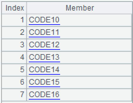
A2: Import D1.ctx and get the sequence of CODE field values. The result is as follows:
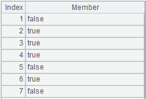
A3: For each value in A2 from the beginning, set the corresponding sequence numbers of CODE values defined in parameter arg_F1 as true if they can be found, and false if they cannot. As the parameter is ordered, we can use contain@b to do the binary search. The result is as follows:
A4: Define the filtering operation before generating a cursor through a Boolean dimension sequence. Below is the filtering process:
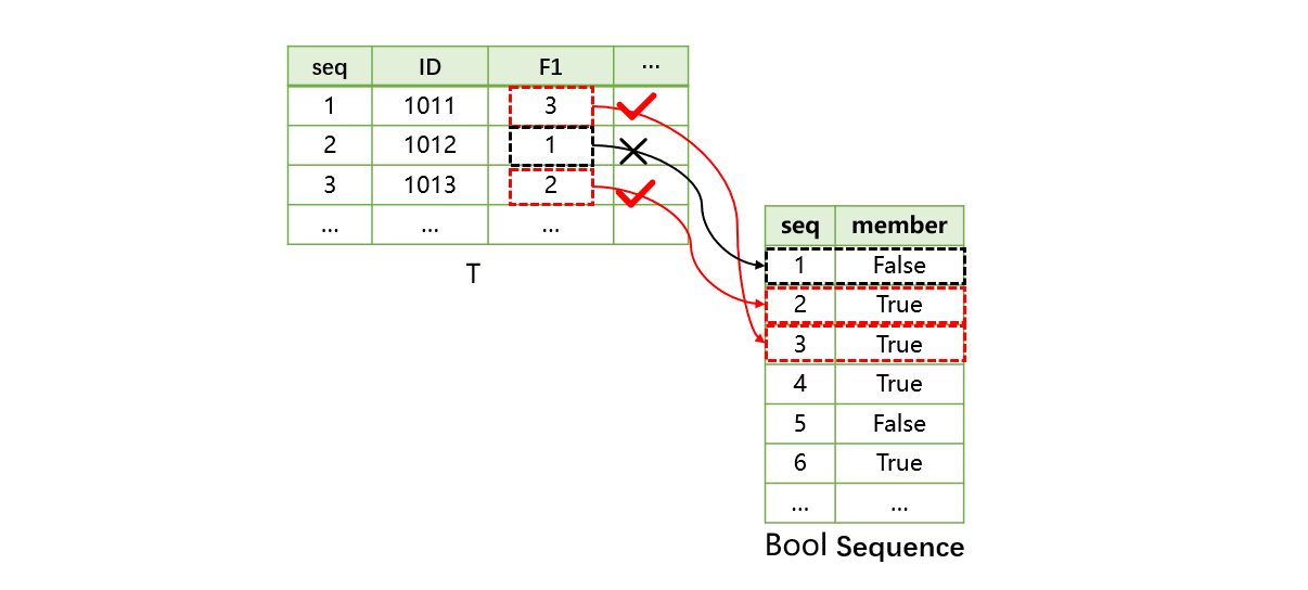
For the first record, the F1 field value, 3, corresponds to the third member in the Boolean dimension sequence, which is true. So, the record is an eligible one. If the corresponding member is false, the record is an ineligible one. The other records are checked in this way, too.
A5: Perform subsequent computations.
As the set of values passed through parameter arg_F1 is ordered, we can use contain@b to calculate the Boolean dimension sequence through location operation. If the set of values is unordered, we need to perform a sort to enable binary search in the subsequent searches and locations (which are the number of members in the dimension table). Yet the performance boost is far more than the cost of the sort. Fortunately, compared with the later traversal, the parameter processing is not so costly. It is tolerable if no sort is done and contain@b is not used.
If the dimension table is relatively large, we can calculate the Boolean dimension sequence in an inverse way to achieve the ultimate performance possible:
| A | |
|---|---|
| 1 | =file("T.ctx").open() |
| 2 | =file("D1.btx").import@ib(CODE) |
| 3 | =A2.(false) |
| 4 | >arg_F1.(A3(A2.pos@b(~))=true) |
| 5 | =A1.cursor(…;A3('F1')) |
| 6 | … |
A3: Define a sequence of the same length as A2. Its members are all false.
A4: Loop through each member of arg_F1 to find the sequence number of the current member’s corresponding item in A2 and set the member at the same position in A3 as true. The original member in A3 will be unchanged if no corresponding sequence number can be found.
The algorithm returns the same result as the above, but it needs a different number of computations to calculate the Boolean dimension sequence.
Suppose the length of arg_F1 is n and that of D1 is m, then the average number of comparisons in A3 in the previous algorithm is m*log2n. The average number of comparisons in A4 in this algorithm is n*log2m. The latter is much more efficient than the former when m≫n.
SPL Resource: SPL Official Website | SPL Blog | Download esProc SPL | SPL Source Code